Replace Hundreds of Formulas With PivotTables

In Lab 3 we wrote a formula for every total. That does not scale: revenue for four regions, four categories and twenty-four months would be hundreds of formulas. A PivotTable adds up thousands of rows by any column with a few clicks. In Lab 4 we build one PivotTable per question, each with a name, on one sheet.

Step 1: The first PivotTable

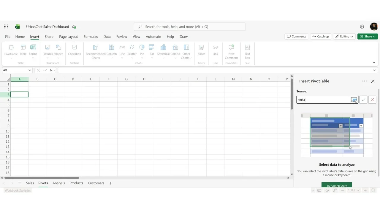
Add a sheet named Pivots, select A3, then Insert → PivotTable. Source: type the table name, tbl_Sales; this is why the data was made a table. Destination: existing sheet, Pivots!A3.

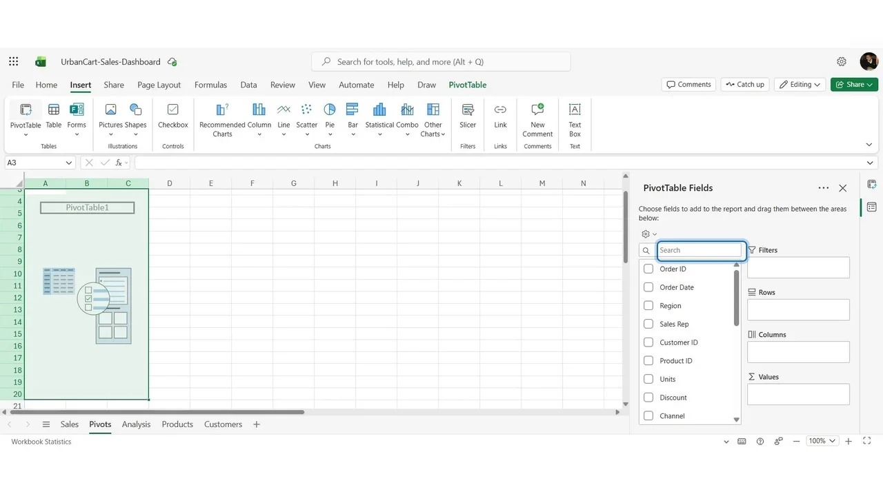
The PivotTable Fields pane: every column at the top, four areas below. Rows: what you compare. Columns: a second split. Values: the numbers. Filters: limit the whole table.

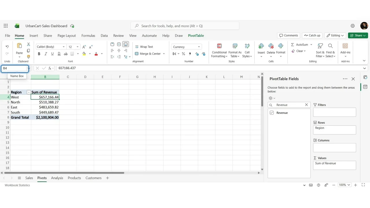
Add Region to Rows and Revenue to Values: four regions and a grand total of $2,100,904, the same total as SUM gave in Lab 3. Name it PVT_Region and sort largest first: West leads with $657,166.

Step 2: The headline numbers

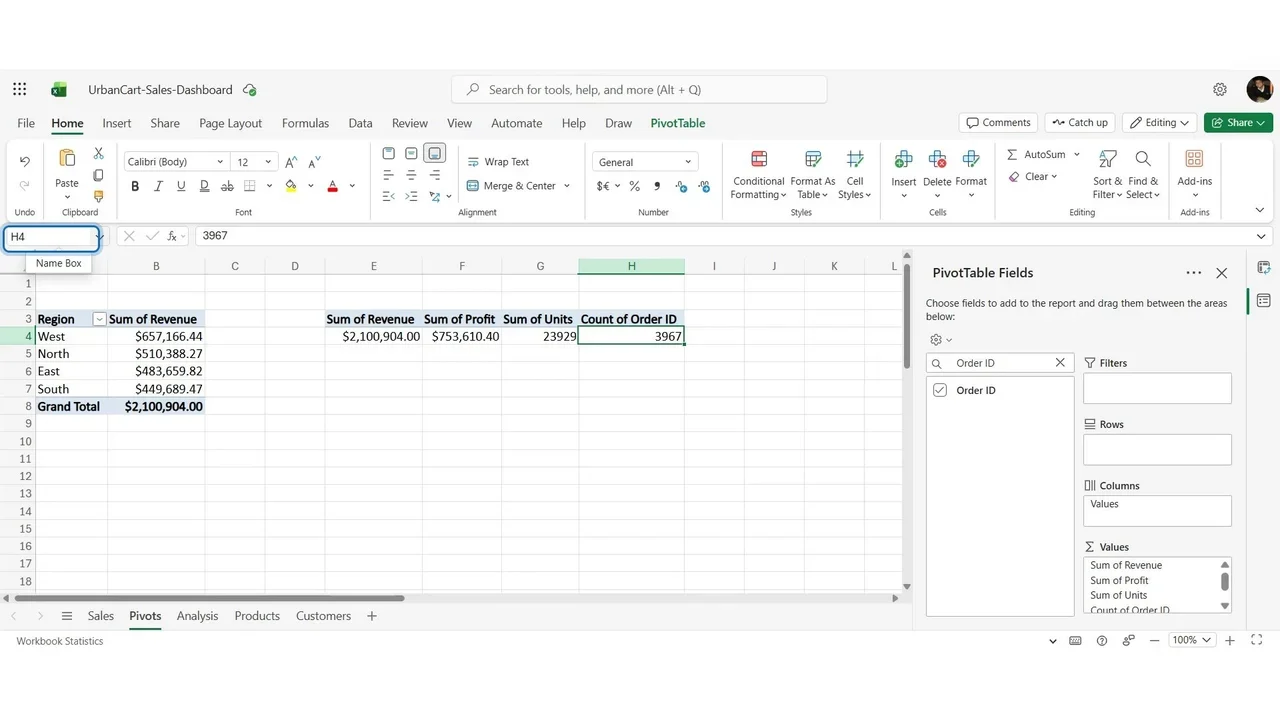
At E3, a PivotTable with no rows, only values: Revenue, Profit, Units, and Order ID, which is text, so Excel counts it. Four numbers in one row: 2,100,904 revenue, 753,610 profit, 23,929 units and 3,967 orders. Name it PVT_KPI; the dashboard cards will read these cells.

Then a PivotTable per Year (use Add to Rows, because a tick would add the years up): 2024 $982,841, 2025 $1,118,063, growth 13.8%, matching the formula from Lab 3.

Step 3: One per chart, and a top 10

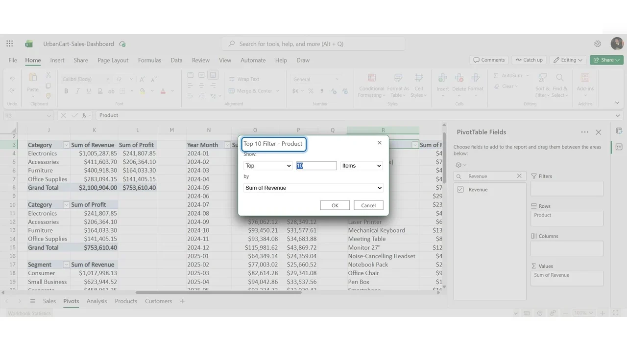
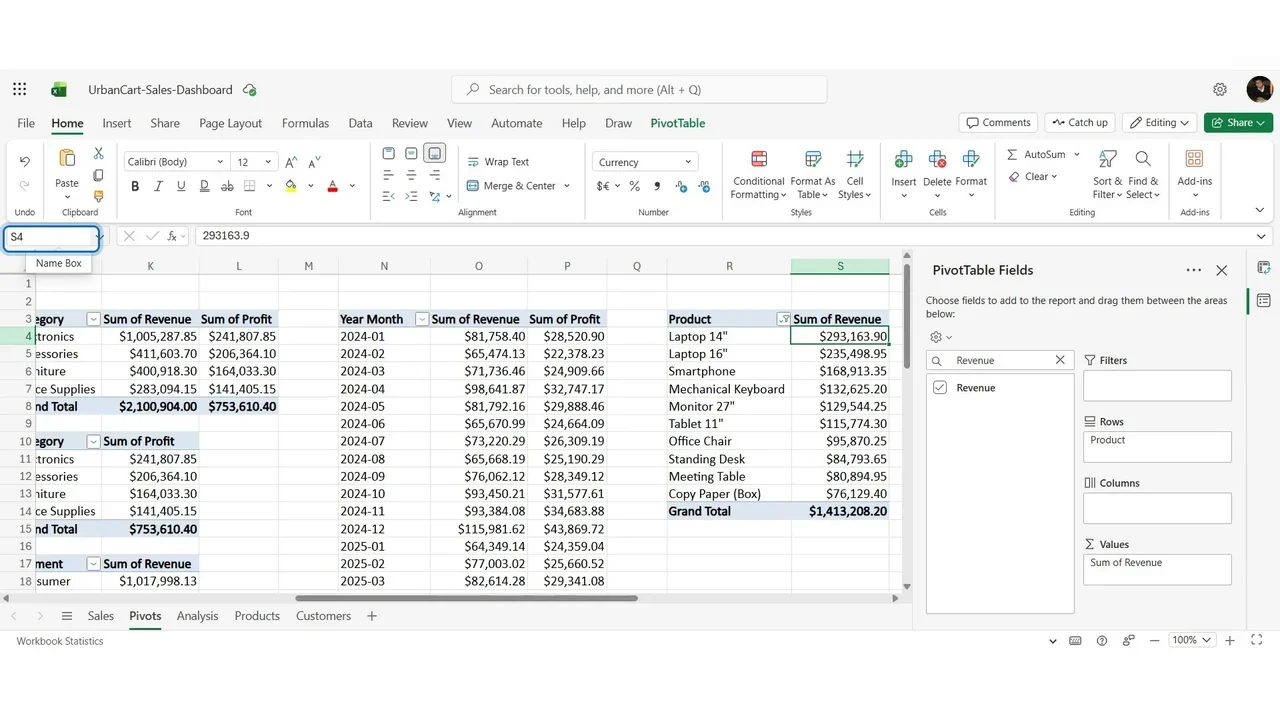
Revenue and profit by category, profit by category alone, revenue by segment, the monthly trend (Year Month sorts correctly because it is year first with two-digit months), and the products. Twenty-four products are too many for a chart: Value Filters → Top 10 by sum of revenue.

How you know it worked

Seven PivotTables on one sheet, each named, each answering one question. Nothing on the sheet is typed by hand, and the totals match the independent formulas from Lab 3.

Tips that save time later

• Name every PivotTable; slicers and GETPIVOTDATA refer to them.
• Leave empty columns between PivotTables, so one can grow without overlapping the next.
• Refresh after new data: the source is a table, so new rows are included.