Build 4 Excel KPI Cards With GETPIVOTDATA

A dashboard opens with a few big numbers. But a number alone says little: two point one million is good news only if last year was lower. In Lab 6 we build four KPI cards, each with a label, a value and a line of context, coloured by rules.

Step 1: A card that reads the PivotTable

A card is a few formatted cells. Merge D5:F5 for the label (Total revenue), and D6:F7 for the value. The formula does not add up the table; it reads the PivotTable:

=GETPIVOTDATA("Sum of Revenue", Pivots!$E$3)

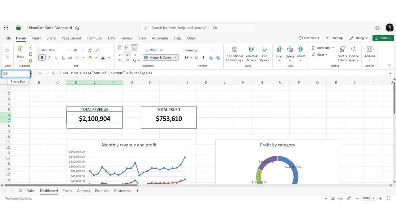
Format it as a headline: currency, no decimals, 20 points, bold, a thin border.

Step 2: Four equal cards

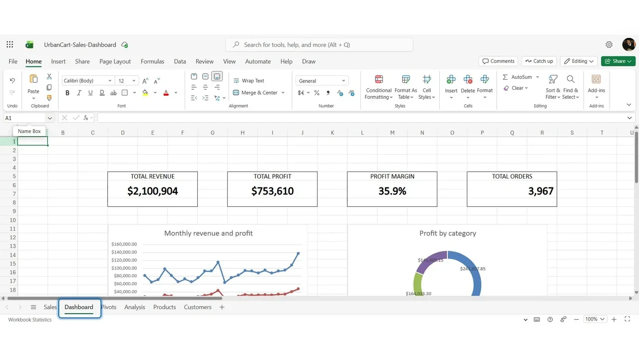
Profit uses the same formula with Sum of Profit. The margin card needs no PivotTable: profit divided by revenue, inside IFERROR so an empty filter shows nothing instead of an error. Orders uses Count of Order ID with a comma style.

Step 3: This year against last year

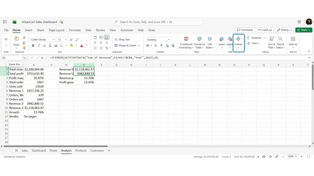
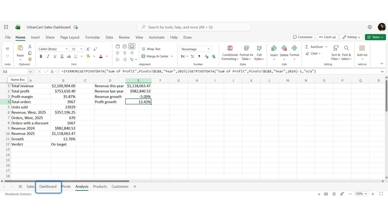
The comparison is a calculation, so it belongs on the Analysis sheet: revenue this year and last year with GETPIVOTDATA filtered by Year, then growth = this year ÷ last year − 1. Revenue grew 13.8%.

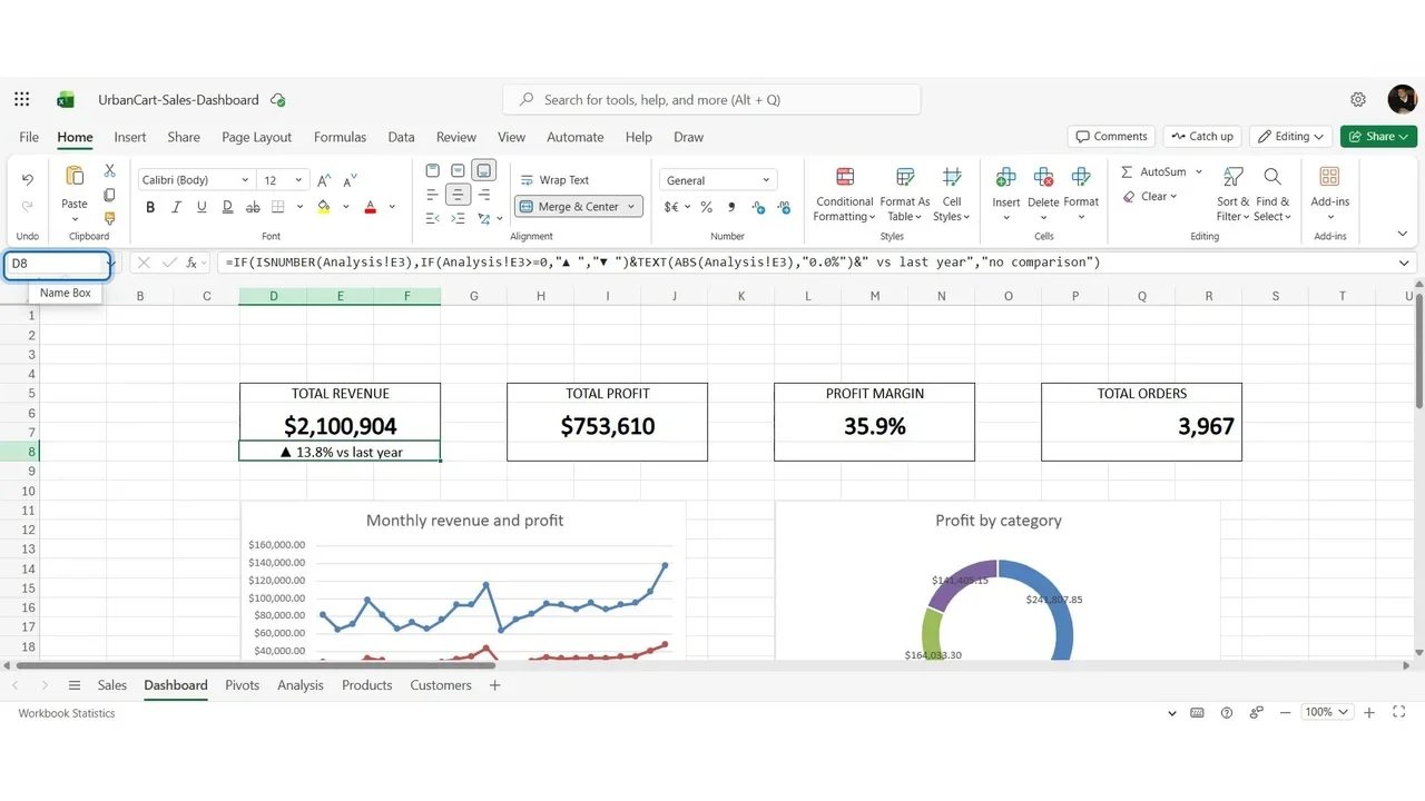
Back on the card, row 8 builds a sentence: an arrow (up when growth is zero or more, down when negative), the percentage, and vs last year.

Step 4: Green and red, by rule

Conditional Formatting → Highlight Cell Rules → Text that Contains the up arrow: green. A second rule for the down arrow: red. And a rule on the margin: less than 30%, red.

How you know it worked

Never trust a rule you have not seen fire. On Analysis, type −5% over the revenue growth for a moment: on the dashboard the arrow turns down and the line turns red. Then put the formula back.

The arrow matters as much as the colour: about one man in twelve does not see the difference between red and green, and the card must still read correctly for them.